In this post, we explore the relationship between Delay Spread in a multipath channel and Coherence Bandwidth of that channel.In a wireless channel, no definite boundaries exist beyond which the signal cannot go. Obstructions in the path of the transmitted waves bounce a part of it away following the laws of reflection. Consequently, at the receiver, multiple versions of the same signal are received which, by virtue of having following different paths, may arrive at different intervals. So, while we transmitted a single beam, what the receiver sees is something like a smudge of different copies of this master signal.
Generally, the greater the number of obstructions that a wave faces, greater is the attenuation. So, beyond a certain point, we cannot detect the contents of the signal in the arriving copies properly. This sets up two time bounds on the signal's arrival. The first bound is the time at which signal arrives at the receiver following the shortest path (or the strongest path which doesn't necessarily have to be the shortest). Let this be \(t_0\) . The second bound is the time of arrival of the last detectable copy of that signal. Let this be denoted by \(t_L\). Then, delay spread is defined as the difference between these two arrivals as \(\tau = t_L - t_o\).

Clearly, the communication system must take this time window into account to avoid mixing of two different signals. If the transmitter were to send the next signal burst with a delay less than the delay spread, there would be smudging of some copies of the first burst with the initial copies of the second burst. This interference of one signal with the other is referred to as inter-symbol interference or ISI. So, to avoid ISI, the system has to be designed keeping in mind the expected delay spreads in the channel.
Another complementary term that is defined is Coherence Bandwidth. It is explained as the range of frequencies which experience more or less the same channel response. This arises from the frequency dual of coherence time. If the bandwidth of the signal is less than the coherence bandwidth, the system is said to have flat fading (that is all frequencies fade similarly). However, if the system bandwidth is greater than the coherence bandwidth, not all frequencies have the same frequency response from the channel and are said to have frequency selective fading. Frequency selective fading is more problematic because we need to find out on a more granular level how the channel affected the signal in that part and compensate for it. That is hard work.
The relationship between Delay spread and Coherence Bandwidth is:
\(B_c = 1/\tau\)
But, how are the two related intuitively? Coherence Bandwidth defines intuitively the range of frequencies that experience the channel in a similar manner. We may say that signals of these frequencies are offered similar resistance by the channel. Hence, over this range of frequencies, the channel response is flat. Delay spread has its own intuitive explanation as the path delays of the first and the last detectable copies of the signal. But can we see how having one fixes the other? Or how changing one affects the other? Sure, we understand the mathematics behind it, but maths models a physical phenomenon here. It would be fun to see how that works. So, we start with a simple mathematical model and start relating it to what the signal experiences.
The signal \(x(t)\) passing through the channel is affected by it. This is captured as the response of the channel as:
\(y(t) = h(t)*x(t)\)
where \(*\) is the linear convolution of the two. \(h(t)\) is the channel's impulse response. Suppose we can cluster the signal copies into L multipath components. Then, we can say that L copies of the signal will be received overall with different delays and gains. The channel response can then be written as:
\(h(t) = \sum_{n=0}^{L-1}a_n\delta(t- \tau_n)\)
where \(a_n\) is the attenuaton factor of the n-th multipath. Finding its frequency response by a Laplace/Fourier transform:
\(H(f) = \int_{-\infty}^{\infty}h(t)e^{-j2\pi ft}.dt\)
using the sampling property of the delta function, this gives:
\(H(f) = \sum_{n=0}^{L-1}a_ne^{-j2\pi f (\tau_n)}\)
which can be written as related to the strongest signal component arriving at \(\tau_o\) as:
\(H(f) =e^{-j2\pi f\tau_0} \sum_{n=0}^{L-1}a_ne^{-j2\pi f(\tau_n - \tau_0)}\)
Then, coherence bandwidth can be written as:
\(B_c = \frac{1}{max(\tau_n) - \tau_0}\)
So, we do see that the two are related somehow, but this is all related to the channel. Sure, the maths is all good, but how does it impact the signal? Let\'s see.
Consider a signal of bandwidth B and lying between frequency \((f_0, f_0+B)\)
Then, we want to see how the value of frequency response varies across this frequency range. We will calculate the channel response at the two edges of our signal bandwidth and see how much different these become as the bandwidth varies. More so, we want to see how large or small the difference becomes without much undulations in between, to check if it is really the case of flat fading within coherence bandwidth and frequency selective fading beyond it. We write an octave/MATLAB program to explore various cases.
%% Explore the variation of channel response across the bandwidth of a signal
f0 = 450e6;
L = 6; %Number of multipaths
delays = sort(1e-6*rand([L,1]), 'ascend');
tau0 = min(delays);
tauN = max(delays);
B_c = 1/(tauN - tau0);
Bandwidths = [0.1, 1, 1.1, 5] .* B_c; %Vary bandwidth of signal according to the coherence bandwidth
ngains = sort([0.9; rand([L-1,1])], 'descend'); %Fixing the first one and letting others vary
figure;
for B_iter = 1:length(Bandwidths)
    B = Bandwidths(B_iter);
    freqs = f0:1:f0+B;
    response = zeros(size(freqs));
    for f= f0:1:f0+B
        response(f-f0+1) = exp(-1j*2*pi*f*tau0)*sum(gains.*exp(-1j*2*pi*f*(delays - tau0)));
    end
    fprintf('Min. Delay: %f Max. Delay: %f Coherence Bandwidth: %f ', tau0, tauN, B_c);
    subplot(2,2, B_iter);
    plot(freqs, abs(response));
    xlabel('Frequency');
    ylabel('Frequency Response');
    legend_str = sprintf('B=%2.2f B_c', B/B_c);
    legend(legend_str);
end
Playing around with the bandwidth parameter of the signal 'B', we can see how the gain varies massively (see the difference of values on the y-axis) when signal bandwidth is comparable to or larger than the coherence bandwidth. In the plots below, the maximum delay is set to be less than 1 microsecond and the coherence bandwidth comes out to be (approximately) 1.3MHz.
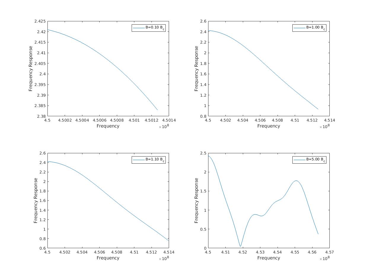
Then, when the signal bandwidth is very small (\(B \ll B_c\)), the channel response can be approximated as flat for the entire signal. At higher bandwidths, we will have to partition the signal into small chunks of flat responses like a staircase function and then estimate each partition's gain and correct the distortion.
To summarize, we see that the delay-spread, which is a function of the channel (inclusive of all the obstructions) determines the coherence-bandwidth of that channel. So, during a communication system design, we have to take both of them into consideration:
- Use a signal bandwidth less than the coherence bandwidth to avoid frequency-selective frequency response from the channel. This simplifies receiver design a bit.
- Have a delay between signal bursts that is greater than the delay spread of the channel. One immediate consequence of this is that signals with long symbol duration (and hence, smaller bandwidth) become preferred.