The Pythagorean Theorem of Statistics

Quick. What’s the most important theorem in statistics? That’s easy. It’s the central limit theorem (CLT), hands down. Okay, how about the second most important theorem? I say it’s the fact that for the sum or difference of independent random variables, variances add:

I like to refer to this statement as the Pythagorean theorem of statistics for several reasons:

1. When written in terms of standard deviations, it looks like the Pythagorean theorem:
   .
2. Just as the Pythagorean theorem applies only to right triangles, this relationship applies only to independent random variables.
3. The name helps students remember both the relationship and the restriction.

As you may suspect, this analogy is more than a mere coincidence. There’s a nice geometric model that represents random variables as vectors whose lengths correspond to their standard deviations. When the variables are independent, the vectors are orthogonal. Then the standard deviation of the sum or difference of the variables is the hypotenuse of a right triangle.

You probably won’t discuss orthogonal vectors with your AP Statistics students, but that’s no excuse for not giving the Pythagorean theorem the emphasis it deserves. When your students understand and learn to use this theorem, many doors open. They gain important insights in dealing with binomial probabilities, inference, and even the CLT itself — and they gain an important problem-solving skill sure to pay off on the AP Exam.

Some Questions

Let’s start by taking a look at the theorem itself. Three questions come to mind:

1. Why do we add the variances?
2. Why do we add even when working with the difference of the random variables?
3. Why do the variables have to be independent?

I’ll answer these questions on two levels. On one level is the proof, just to make you feel better. Although some teachers may decide to show this proof to their classes, most won’t inflict it on AP Statistics students. Instead, a plausibility argument should suffice. By that I mean a series of justifications that stop short of being formal proofs yet give students clear examples that make the theorem something believable and vital, not simply a meaningless rule to memorize.

Proving the Theorem: The Math

First, then, let’s have a look at a formal proof. It’s a rule of mathematics that no proof should be taken seriously unless there’s a lemma, so here’s ours. The proof uses the fact that, because expected values are basically summations, they are additive:

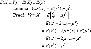
And now, the Pythagorean theorem of statistics:

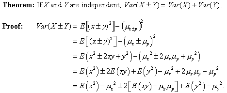
Consider that middle term: E(xy) - µ_xµ_y.

E(xy) is the sum of all terms of the form x_iy_j·P(x_i ∩ y_j). The product µ_xµ_y is the sum of all terms of the form x_iP(x_i) · y_jP(y_j). If X and Y are independent, each term in the first sum is equal to the corresponding term in the second sum; hence that middle term is 0. Thus:

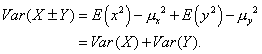
Note that this proof answers all three questions we posed. It’s the variances that add. Variances add for the sum and for the difference of the random variables because the plus-or-minus terms dropped out along the way. And independence was why part of the expression vanished, leaving us with the sum of the variances.

Teaching the Theorem

Although that proof may make you feel better about the theorem (or not), it’s not likely to warm the hearts of most of your students. Let’s have a look at some arguments you can make in class that show your students the theorem makes sense.

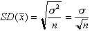
Question 1: Why add variances instead of standard deviations?
We always calculate variability by summing squared deviations from the mean. That gives us a variance—measured in square units (square dollars, say, whatever those are). We realign the units with the variable by taking the square root of that variance. This gives us the standard deviation (now in dollars again). To get the standard deviation of the sum of the variables, we need to find the square root of the sum of the squared deviations from the mean. Students have learned in algebra that they shouldn’t add the square roots, because .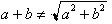

Although 3 + 4 = 7, we need , the Pythagorean approach. We add the variances, not the standard deviations.

Question 2: Why add even for the difference of the variables?
We buy some cereal. The box says “16 ounces.” We know that’s not precisely the weight of the cereal in the box, just close. After all, one corn flake more or less would change the weight ever so slightly. Weights of such boxes of cereal vary somewhat, and our uncertainty about the exact weight is expressed by the variance (or standard deviation) of those weights.

Next we get out a bowl that holds 3 ounces of cereal and pour it full. Our pouring skill is not very precise, so the bowl now contains about 3 ounces with some variability (uncertainty).

How much cereal is left in the box? Well, we assume about 13 ounces. But notice that we’re less certain about this remaining weight than we were about the weight before we poured out the bowlful. The variability of the weight in the box has increased even though we subtracted cereal.

Moral: Every time something happens at random, whether it adds to the pile or subtracts from it, uncertainty (read “variance”) increases.

Question 2 (follow-up): Okay, but is the effect exactly the same when we subtract as when we add?
Suppose we have some grapefruit weighing between 16 and 24 ounces and some oranges weighing between 9 and 13 ounces. We pick one of each at random.

• Consider the total possible weight of the two fruits. The maximum total is 24 + 13 = 37 ounces, and the minimum is 16 + 9 = 25 ounces – a range of 12 ounces.
• Now consider the possible weight difference. The maximum difference is 24 - 9 = 15 ounces, and the minimum is 16 - 13 = 3 ounces—again a range of 12 ounces. So whether we’re adding or subtracting the random variables, the resulting range (one measure of variability) is exactly the same. That’s a plausibility argument that the standard deviations of the sum, and the difference should be the same, too.

Question 3: Why do the variables have to be independent?
Consider a survey in which we ask people two questions:

• During the last 24 hours, how many hours were you asleep?
• And how many hours were you awake?

There will be some mean number of sleeping hours for the group, with some standard deviation. There will also be a mean and standard deviation of waking hours. But now let’s sum the two answers for each person. What’s the standard deviation of this sum? It’s 0, because that sum is 24 hours for everyone—a constant. Clearly, variances did not add here.

Why not? These data are paired, not independent, as required by the theorem. Just as we can’t apply the Pythagorean theorem without first being sure we are dealing with a right triangle, we can’t add variances until we’re sure the random variables are independent. (This is yet another place where students must remember to check a condition before proceeding.)

Why Does It Matter?

Many teachers wonder if teaching this theorem is worth the struggle. I say getting students to understand this key concept (1) is not that difficult and (2) pays off throughout the course, on the AP Exam, and in future work our students do in statistics. In fact, it comes up so often that the statement “For sums or differences of independent random variables, variances add” is a mantra in my classroom. Let’s take a tour of some of the places the Pythagorean theorem of statistics holds the key to understanding.

Working with Sums

Remember Matt and Dave’s Video Venture, a multiple-choice question from the 1997 AP Exam? At Matt and Dave’s, every Thursday was Roll-the-Dice Day, allowing patrons to rent a second video at a discount determined by the digits rolled on two dice. Students were told that these second movies would cost an average of $0.47, with a standard deviation is $0.15. Then they were asked:

If a customer rolls the dice and rents a second movie every Thursday for 30 consecutive weeks, what is the approximate probability that the total amount paid for these second movies will exceed $15.00?

One route to the solution adds variances.

First we note that the total amount paid is the sum of 30 daily values of a random variable.

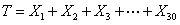
We find the expected total.

Because rolls of the dice are independent, we can apply the Pythagorean theorem to find the variance of the total, and that gives us the standard deviation.

The CLT tells us that sums (essentially the same thing as means) of independent random variables approach a normal model as n increases. With n = 30 here, we can safely estimate the probability that T > 15.00 by working with the model N(14.10, 0.822).

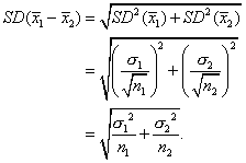
Working with Differences

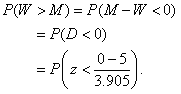
On the 2000 AP Exam, the investigative task asked students to consider heights of men and women. They were given that the heights of each sex are described by a normal model. Means were given as 70 inches for men and 65 inches for women, with standard deviations of 3 inches and 2.5 inches, respectively. Among the questions asked was:

Again, we can solve the problem by adding variances:

First, define the random variables.

M = Height of the chosen man, W = Height of the woman.

We’re interested in the difference of their heights.

Let D = Difference in their heights: D = M - W.

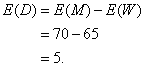
Because the people were selected at random, the heights are independent, so we can find the standard deviation of the difference using the Pythagorean theorem.

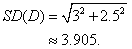
The difference of two normal random variables is also normal, so we can now find the probability that the woman is taller using the z-score for a difference of 0.

Standard Deviation for the Binomial

How many 4s do we expect when we roll 600 dice? 100 seems pretty obvious, and students rarely question the fact that for a binomial model µ = np. However, the standard deviation is not so obvious. Let’s derive that formula.

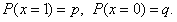
We start by looking at a probability model for a single Bernoulli trial.

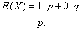
Let X = the number of successes.

We find the mean of this random variable.

And then the variance.

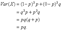
Now we count the number of successes in n independent trials.

The mean is no surprise.

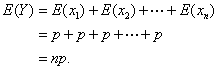
And the standard deviation? Just add variances.

The Central Limit Theorem

By using the second most important theorem in statistics, we can derive part of the most important theorem. The central limit theorem (CLT) tells us something quite surprising and beautiful: When we sample from any population, regardless of shape, the behavior of sample means (or sums) can be described by a normal model that increases in accuracy as the sample size increases. The result is not just stunning, it’s also quite fortunate because most of the rest of what we teach in AP Statistics would not exist were it not true.

The full proof of the CLT is well beyond the scope of this article. What’s within our grasp is the theorem’s quantification of the variability in these sample means, and the key is (drum roll!) adding variances.

The mean is basically the sum of n independent random variables, so:

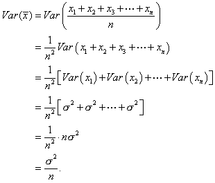
Hence,

Inference for the Difference of Proportions

The Pythagorean theorem also lets students make sense of those otherwise scary-looking formulas for inferences involving two samples. Indeed, I’ve found that students can come up with the formulas for themselves. Here’s how that plays out in my classroom.

To set the stage for this discussion, we’ve just started inference. We first developed the concept of confidence intervals by looking at a confidence interval for a proportion. We then discussed hypothesis tests for a proportion, and we’ve spent a few days practicing the procedures. By now students understand the ideas and can write up both a confidence interval and a hypothesis test, but only for one proportion. When class starts, I propose the following scenario:

We begin by drawing a flowchart for the experiment – a good review lesson. Start with a cohort of volunteer smokers trying to quit. Randomly divide them into two groups. Both groups get the patch. One group also attends these support/counseling sessions. Wait six months. Then compare the success rates in the two groups.

Earlier in the course, this is where the discussion ended, but now we are ready to finish the job and “compare the success rates”:

Students recognize that we need to test a hypothesis, and they point out that this is a different situation because there are two groups. I bet them they can figure out how to do it, and I start writing their suggestions on the board. They propose a hypothesis that the success rates are the same:

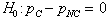
I agree, and then I add that we may also write this hypothesis as a statement of no difference:

They dictate the randomization, success/failure, and 10 percent conditions that allow the use of a normal model. They compute the sample proportions and find the observed difference,

Here’s where it gets interesting. They need to find the probability of observing a difference in proportions at least as large as 0.123, when they were expecting a difference of zero.

They start to find the z-score, , but they get stumped by the denominator. I wait. If necessary, I point out that we need to find the standard deviation of the difference of the sample proportions. Soon someone gets it: “Add the variances!”

Good idea, but can we add the variances? Only if the groups are independent. Why are they independent? Randomization! We return to the list of conditions and add one more: the independent group’s condition. At this point, rather than memorizing a list of conditions, everyone clearly realizes why this condition must be met.

Next we look at what happens when we add the variances:

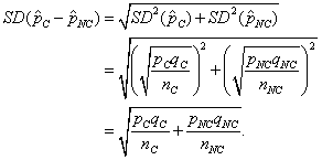
Voila! The students have derived the formula for the standard deviation of the difference of sample proportions; thus it makes sense to them. We still need to talk about issues like using the sample proportions as estimates and pooling, but the basic formula is at hand and understood.

Inference for the Difference of Means

There’s no need to give you a long-winded example that’s analogous to the situation for proportions. It’s enough to see that the standard deviation for the difference of sample means is also based on adding variances. And it’s clear that students can derive it on their own the first time you test a hypothesis about the difference of means of independent groups:

Two-Sample t-Procedures, or Matched Pairs – It Matters!

Without advance fanfare, I propose to the class that we construct a confidence interval to see how many extra miles per gallon we might get if we use premium rather than regular gasoline. I give the students data from an experiment that tried both types of fuel in several cars (a situation involving matched pairs, but I don’t point that out). When we start constructing the confidence interval, invariably someone questions the assumption that two measurements made for the same car are independent. I insist students explain why that matters. The insight that lack of independence prevents adding variances, which in turn renders the formula for a two-sample t-interval incorrect, makes it forever clear to students that they must think carefully about the design under which their data were collected before plunging into the analysis. There’s never a “choice” whether to use a paired differences procedure or a two-sample t-method.

Create One Confidence Interval, or Two?

	Diet S	Diet N
n	36	36
Mean	55 lbs.	53 lbs.
SD	3 lbs.	4 lbs.

Suppose we wonder if a food supplement can increase weight gain in feeder pigs. An experiment randomly assigns some pigs to one of two diets, identical except for the inclusion of the supplement in the feed for Group S but not for Group N. After a few weeks, we weigh the pigs; summaries of the weight gains appear in the table. Is there evidence that the supplement was effective? A reasonable way to try to answer this question is by using confidence intervals, but which approach is correct?

Plan A: Compare confidence intervals for each group. The separate intervals indicate we can be 95 percent confident that pigs fed this dietary supplement for this period of time would gain an average of between 53.90 and 56.01 pounds, while the average gain for those not fed the supplement would be between 51.65 and 54.35 pounds.

Note that these intervals overlap. It appears to be possible that the two diets might result in the same mean weight gain. Because of this, we lack evidence that the supplement is effective.

Plan B: Construct one confidence interval for the difference in mean weight gain. We can be 95 percent confident that pigs fed the food supplement would gain an average of between 0.34 and 3.66 pounds more than those that were not fed this supplement. Because 0 is not in this confidence interval, we have strong evidence that this food supplement can make feeder pigs gain more weight.

The conclusions are contradictory, but it may not be immediately obvious which is correct. Students often see nothing wrong with Plan A. Such a conclusion would be inaccurate. Whether the two intervals overlap depends on whether the two means are farther apart than the sum of the margins of error. The mistake rests in the fact that we shouldn’t add the margins of error. Why not? A confidence interval’s margin of error is based on a standard deviation (well, standard error to be more exact). But standard deviations don’t add; variances do. Plan B’s confidence interval for the difference bases its margin of error on the standard error for the difference of two sample means, calculated by adding the two variances. That’s the correct approach — one confidence interval, not two.

Future Encounters

Even if you’ve sometimes been stuck in the discussion this far, you should at the very least be convinced that adding variances plays a key role in much of the statistics we teach in the AP course. As our students expand their knowledge of statistics by taking more courses beyond AP Statistics, they encounter the Pythagorean theorem again and again. To cite a few places on the horizon:

• Prediction intervals: When we use a regression line to make a prediction, we should include a margin of error around our estimate. That uncertainty involves three independent sources of error: (1) the line may be misplaced vertically because our sample mean only approximates the true mean of the response variable, (2) our sample data only gives us an estimate of the true slope, and (3) individuals vary above and below the line.
• Multiple regression: When we use several independent factors to arrive at an estimate for the response variable, we assess the strength of the model by looking at the total amount of variability it explains. We’re further able to attribute some of that variability to each of the explanatory variables.
• ANOVA: As the name “analysis of variance” suggests, we compare the effects of treatments on multiple groups or assess the effects of several treatments in a multifactor design by comparing the variability seen within groups to the total variability across groups. Here again, the idea of adding variances lies at the heart of the statistics.

Let’s summarize: Variances add. And yes, it matters!